Quickstart Guide for MINT

Welcome to the MINT quickstart guide! This guide helps you get up and running with the application so you can start analyzing mass spectrometry data efficiently. Follow the steps below to install the app, create a workspace, and begin processing your data.

1. Install and Open `MINT`

Install MINT (see installation options here) or download an executable compatible with your OS. Once the app starts, you should see the Workspaces tab.

2. Create a workspace

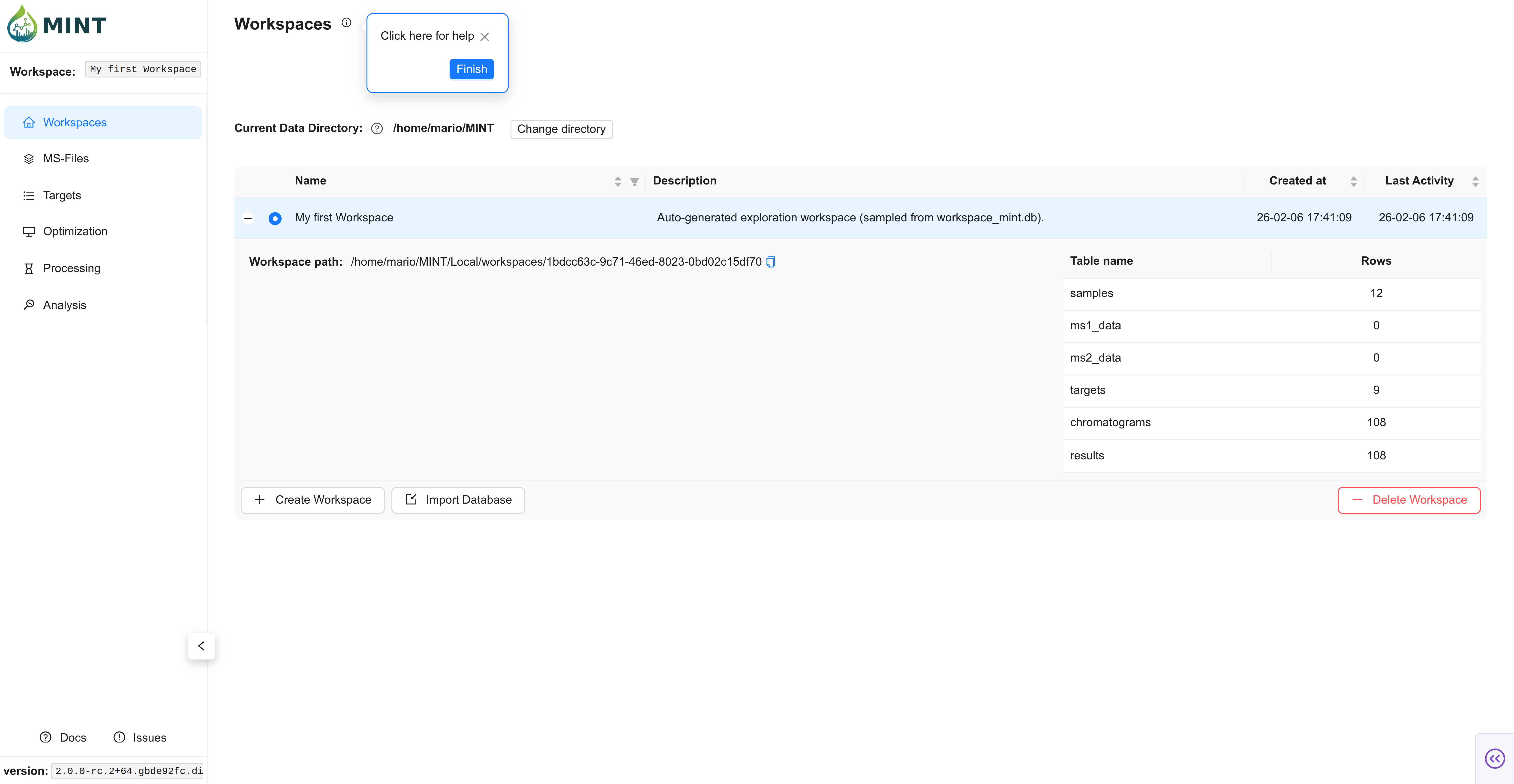
On first launch, MINT creates a My first Workspace workspace with test data so you can tour the interface immediately. You can keep it for reference or create a new workspace for your project. A workspace provides easy access to all data files and results for a given project.

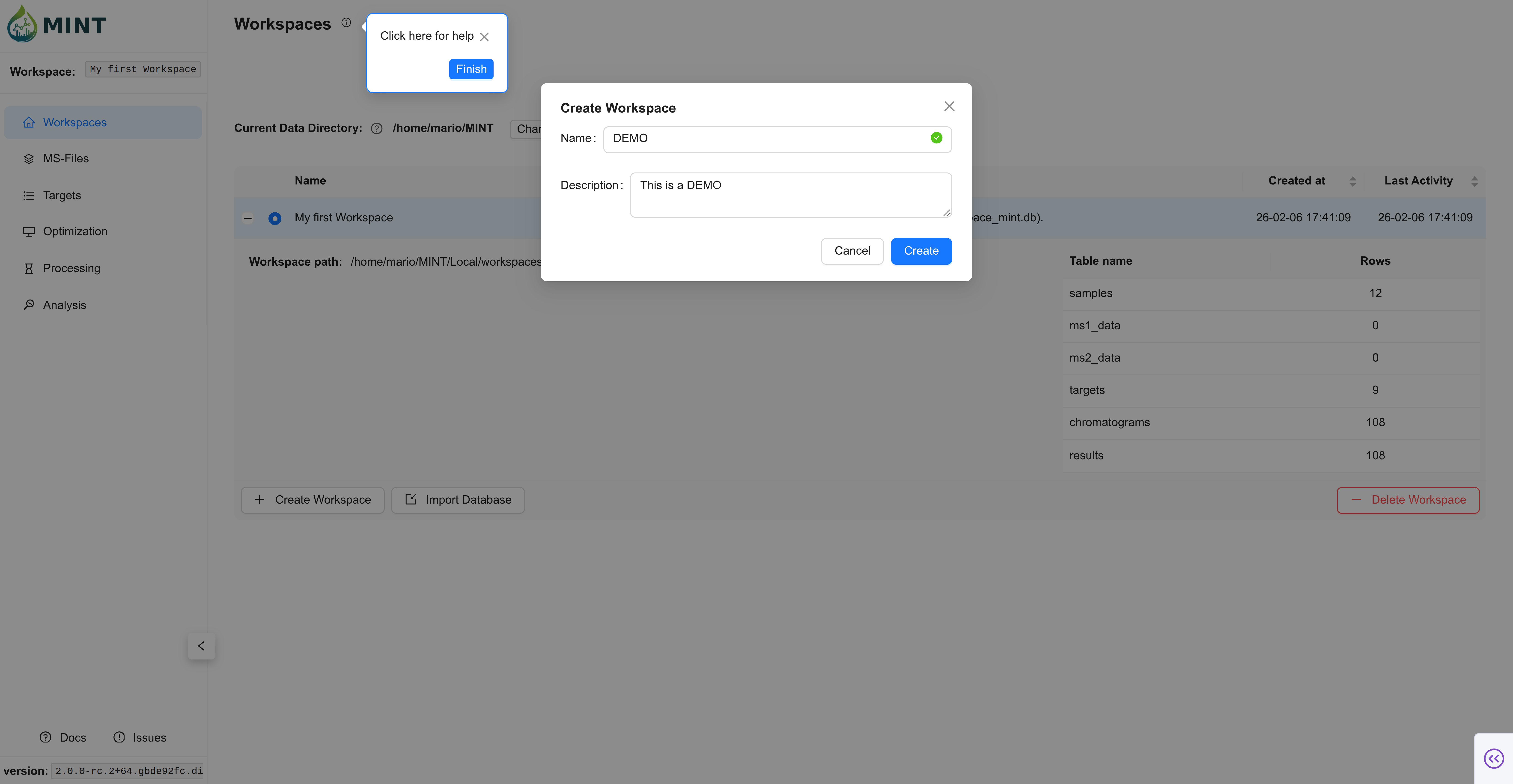
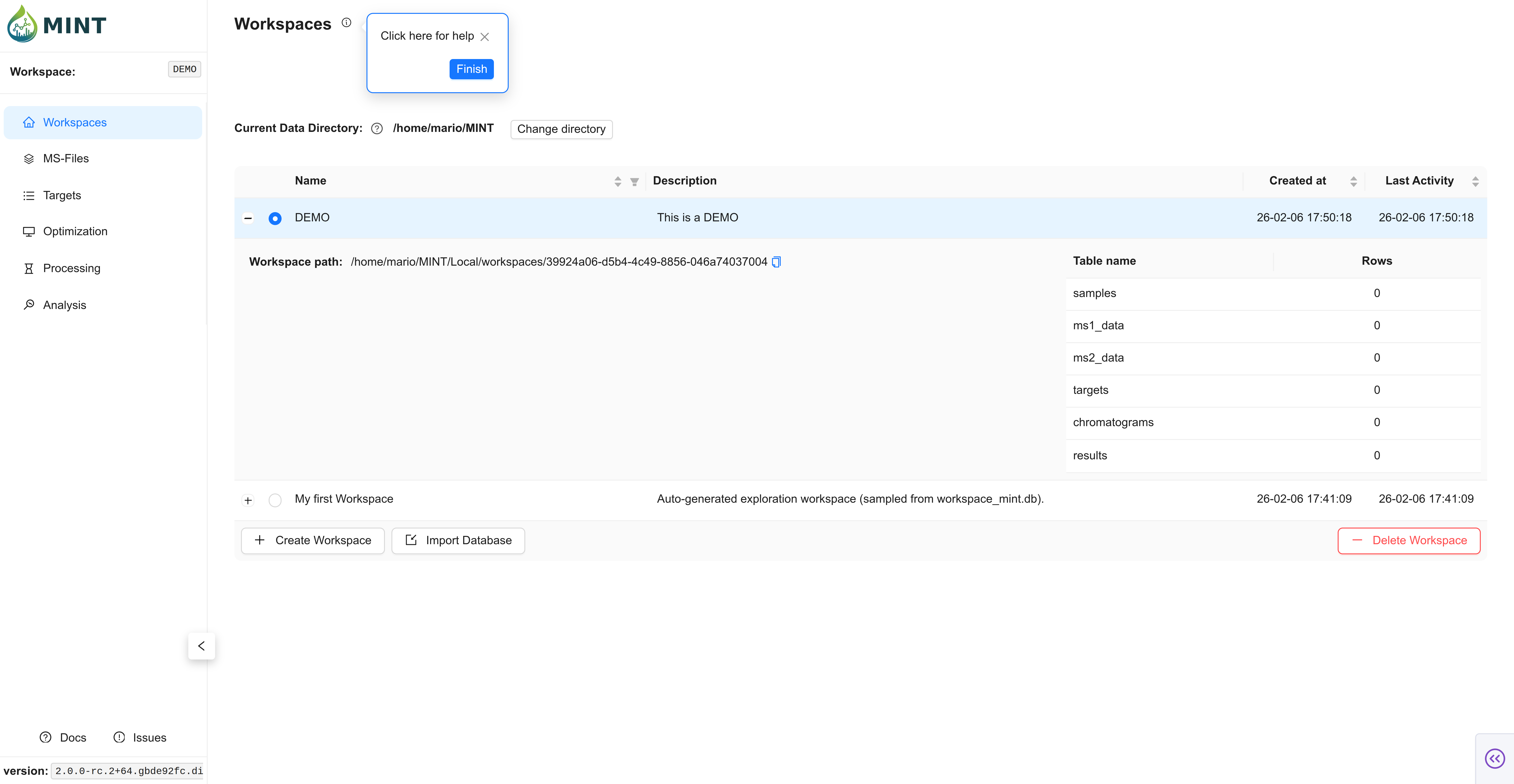
In the Workspaces tab, click the + Create Workspace button. A dialog opens asking for the name of the workspace and an optional description. Type DEMO into the text field, add a brief description like This is a DEMO, and click Create. Expected result: the DEMO workspace appears with a blue toggle indicating it is active.

You can see which workspace is active by looking at the blue toggle to the left of the workspace name. Click the + sign to view the workspace folder location and stats like how many samples were analyzed and how many compounds were included in the analysis.

Now you have created your first workspace, but it is empty. You will need some input files to populate it.

3. Download the demo files

If you only want to explore the UI quickly, you can use the pre-seeded My first Workspace workspace and jump ahead to the analysis section. For a full end-to-end walkthrough with real files, download the demo files below.

Some demo files are available for download on the MINT GitHub repository. Download the files from here and extract the archive.

This is the directory tree of the demo files:

.
├── metadata
│   ├── metadata.csv
├── ms-files
│   ├── CA_B1.mzXML
│   ├── CA_B2.mzXML
│   ├── CA_B3.mzXML
│   ├── CA_B4.mzXML
│   ├── EC_B1.mzXML
│   ├── EC_B2.mzXML
│   ├── EC_B3.mzXML
│   ├── EC_B4.mzXML
│   ├── SA_B1.mzML
│   ├── SA_B2.mzML
│   ├── SA_B3.mzML
│   └── SA_B4.mzML
└── targets
    ├── targets.csv
    └── targets_template.csv

3 directories, 15 files

A folder (ms-files) with 12 mass spectrometry (MS) files from microbial samples. We have four files for each Escherichia coli (EC), Candida albicans (CA), and Staphylococcus aureus (SA). Each file belongs to one of four batches (B1-B4).
A folder (metadata) with a metadata.csv file containing this information in tabular format. Submitting metadata is optional, but highly recommended to make downstream analysis smoother.
A folder (targets) with a targets.csv file containing the extraction lists. The identification of the metabolites has been done before, so we know where the metabolites appear in the MS data.

4. Upload LC-MS files

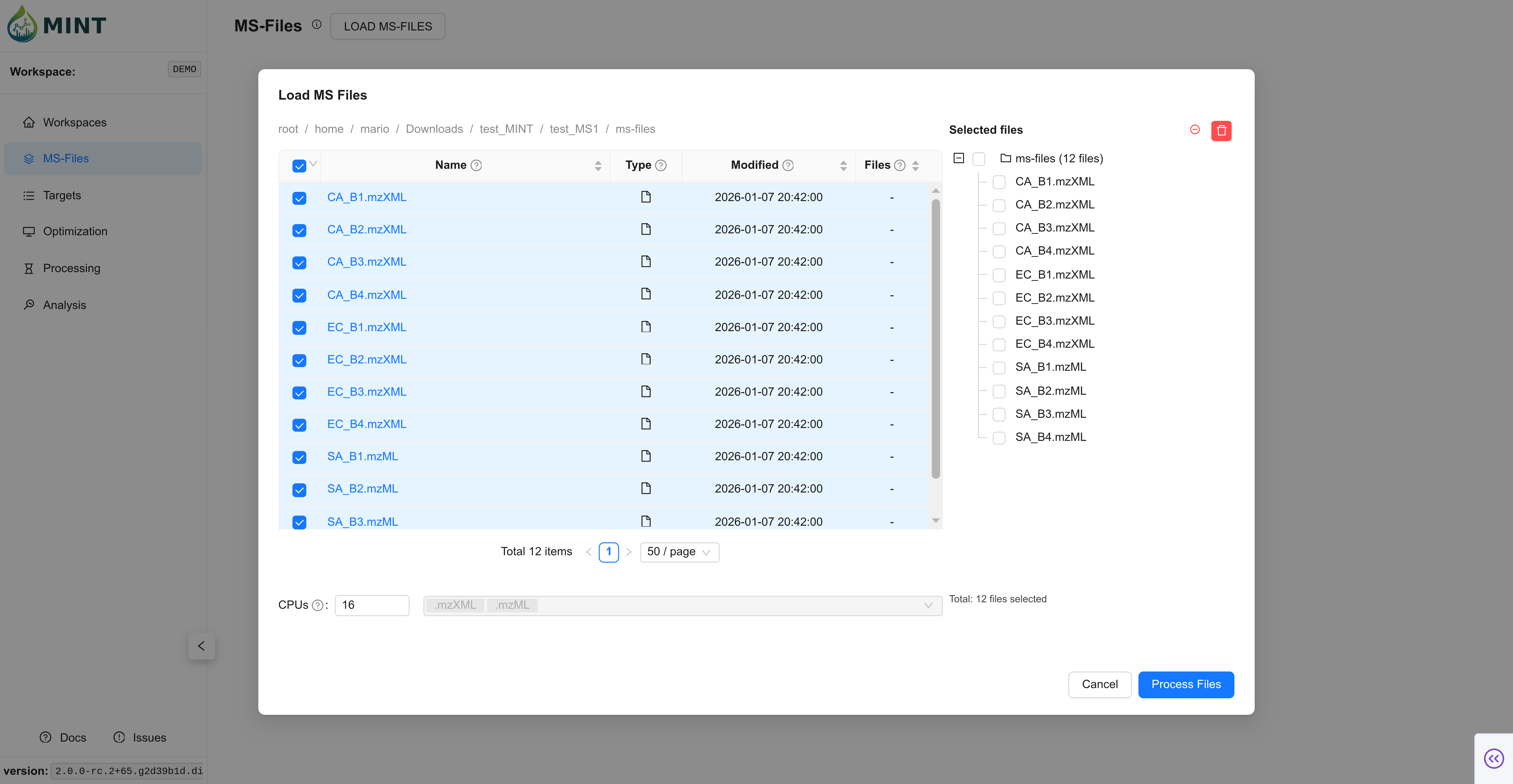
Switch to the MS-Files tab and upload the 12 MS files. Click LOAD MS-FILES, navigate to the folder where the files are located, select either the files individually or the folder, and click Process Files. Expected result: the 12 files appear in the MS-Files table.

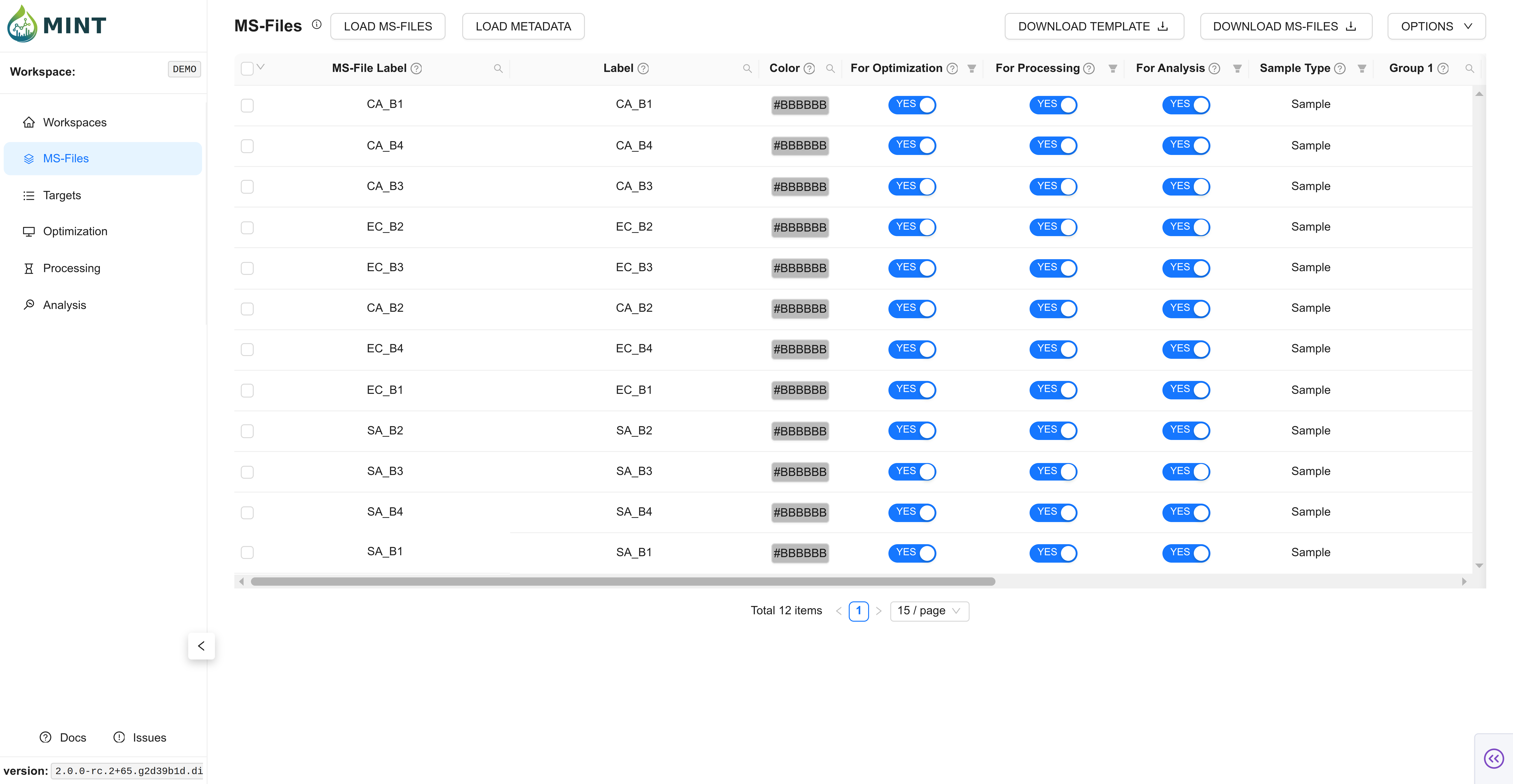
At this point you can proceed with the rest of the steps without providing any metadata; however, we strongly recommend using metadata to streamline downstream analyses.

5. Add metadata (Optional, but highly recommended)

In the same way as before, click LOAD METADATA on the top left, navigate to the folder where the metadata file is located, select the file, and click Process Files. If colors are not provided, automatic ones are assigned according to sample type.

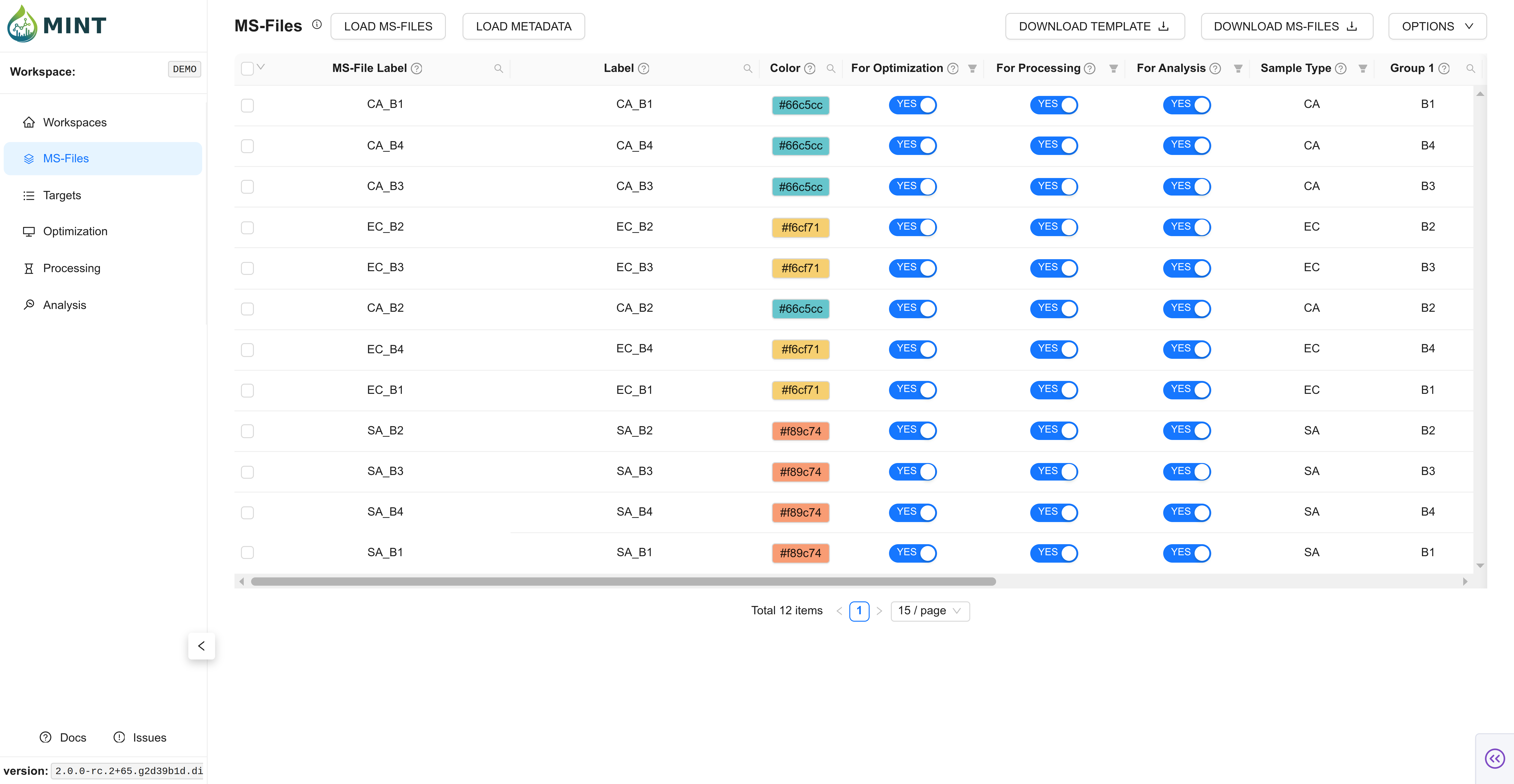
This file contains important information about your samples. Only ms_file_label and sample_type are essential; the remaining columns are optional but useful for grouping and plotting. If any of the columns use_for_optimization, use_for_processing, use_for_analysis are left blank they will be assumed to be TRUE.

Column Name	Description
`ms_file_label`	Unique file name; must match the MS file on disk
`label`	Friendly label to display in plots and reports
`color`	Hex color for visualizations (auto-generated if blank)
`use_for_optimization`	True to include in optimization steps (COMPUTE CHROMATOGRAMS)
`use_for_processing`	True to include in processing (RUN MINT)
`use_for_analysis`	True to include in analysis outputs
`sample_type`	Sample category (e.g.; Sample; QC; Blank; Standard)
`group_1`	User-defined grouping field 1 for analysis/grouping (free text)
`group_2`	User-defined grouping field 2 for analysis/grouping (free text)
`group_3`	User-defined grouping field 3 for analysis/grouping (free text)
`group_4`	User-defined grouping field 4 for analysis/grouping (free text)
`group_5`	User-defined grouping field 5 for analysis/grouping (free text)
`polarity`	Polarity (Positive or Negative)
`ms_type`	Acquisition type (ms1 or ms2)

6. Add targets (metabolites)

Switch to the Targets tab and upload targets.csv. This file is located in the targets folder within the demo archive.

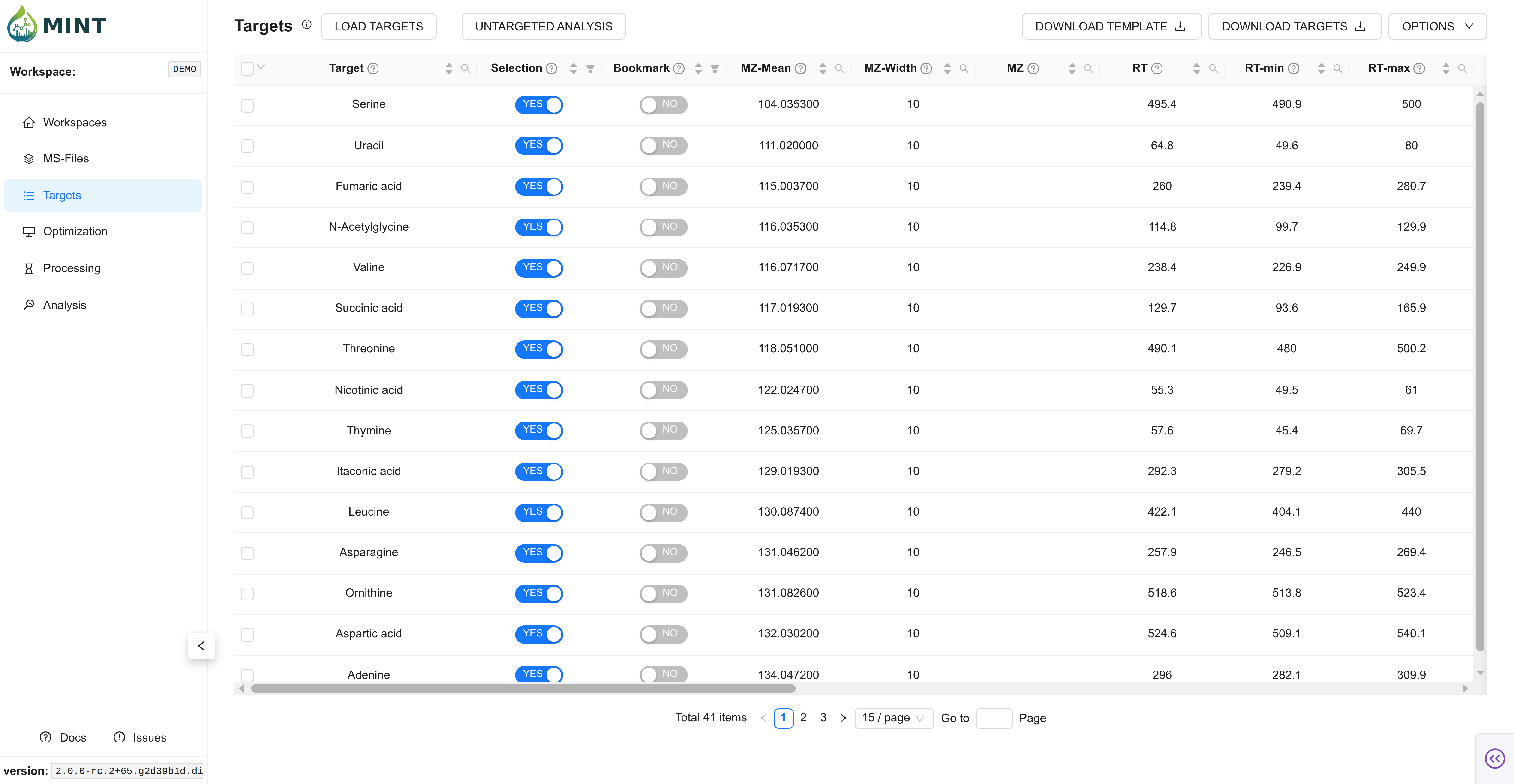
This is the data extraction protocol. It determines what data is extracted from the files. The same protocol is applied to all files. No fitting or peak optimization is done.

After a successful target import, MINT automatically writes a backup snapshot at <workspace>/data/targets_backup.csv. This snapshot is refreshed on later target uploads (or untargeted generation) and can be useful for recovery/export.

This file contains important information about the targets.

Column Name	Description
`peak_label`	Unique metabolite/feature name
`peak_selection`	True if selected for analysis
`bookmark`	True if bookmarked
`mz_mean`	Mean m/z (centroid)
`mz_width`	m/z window or tolerance
`mz`	Precursor m/z (MS2)
`rt`	Retention time (default: in seconds)
`rt_min`	Lower RT bound (default: in seconds)
`rt_max`	Upper RT bound (default: in seconds)
`rt_unit`	RT unit (e.g. s or min; default: in seconds)
`intensity_threshold`	Intensity cutoff (anything lower than this value is considered zero)
`polarity`	Polarity (Positive or Negative)
`filterLine`	Filter ID for MS2 scans
`ms_type`	ms1 or ms2
`category`	Category
`formula`	Chemical formula (used to derive m/z when mz_mean is missing)
`maven_id`	Maven ID or Group ID (optional identifier)
`adduct_name`	Adduct name (e.g. [M+H]+); optional and can be auto-populated
`score`	Optional legacy score field
`notes`	Free-form notes
`source`	Data source or file

7. Optimize retention times (Optional, but highly recommended)

Switch to the Optimization tab. Traditionally, and especially for large datasets, you select a representative set of samples including standards (with known concentrations of the target metabolites) to perform the optimization. However, in MINT, you can perform the optimization with all samples in most cases (see the files selected for optimization in the tree on the left side).

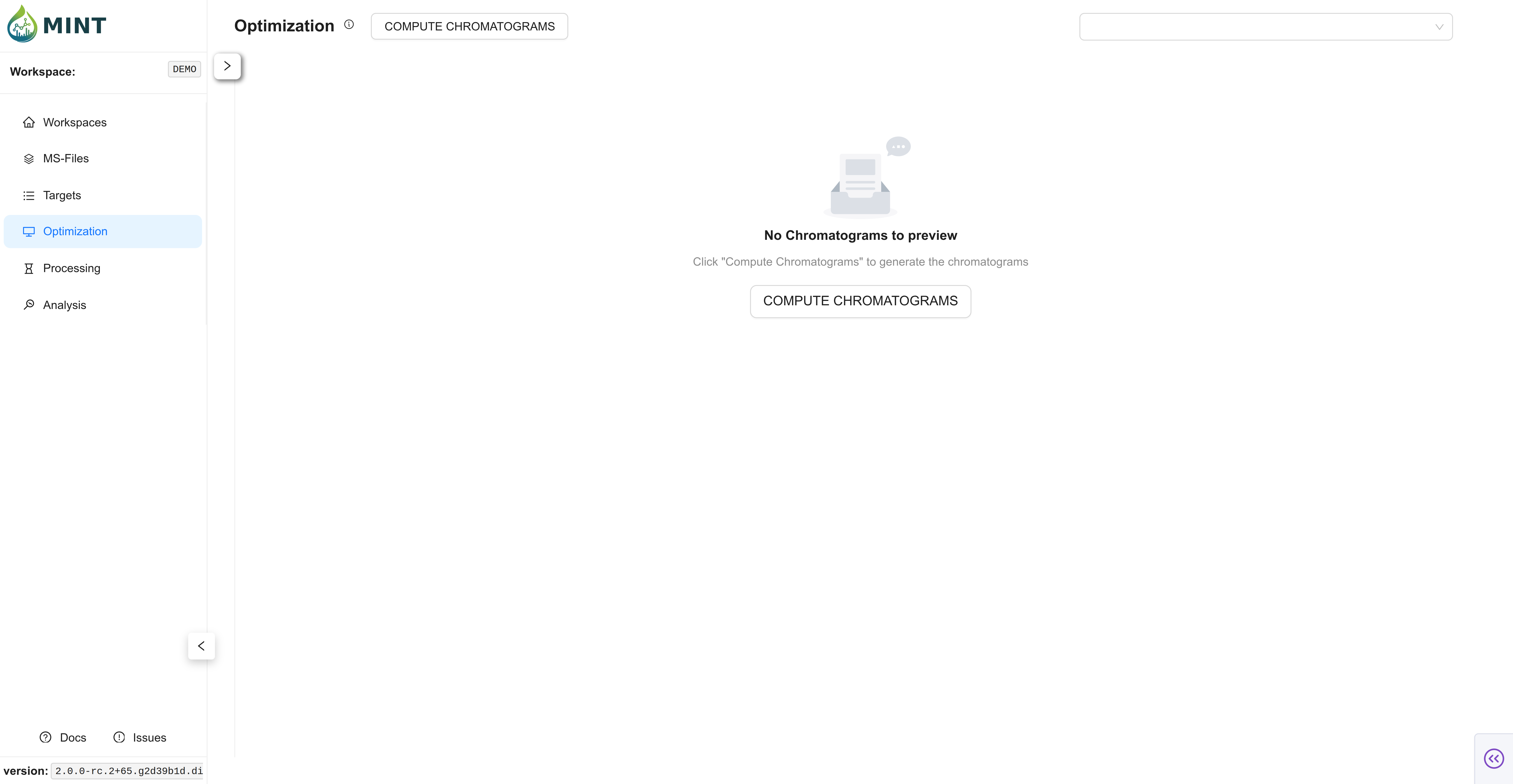
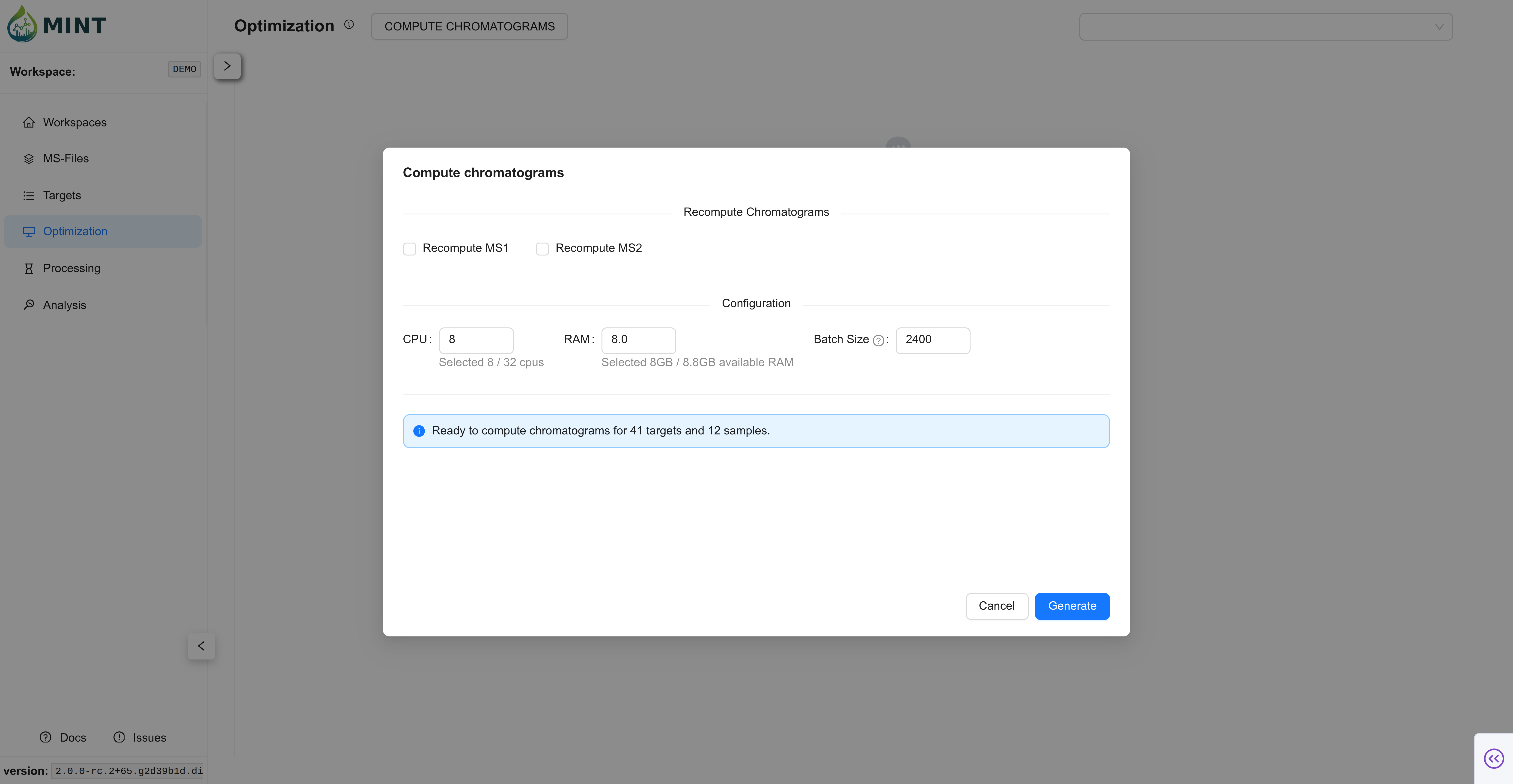
Peak optimization takes longer as you use more files and define more targets. Click COMPUTE CHROMATOGRAMS. Here you can choose how many resources to allocate to process the files, including CPU, RAM, and batch size. In small datasets the default values should suffice; as the number of files used for optimization grows, tweaking these parameters improves performance. Click Generate to compute the chromatograms.

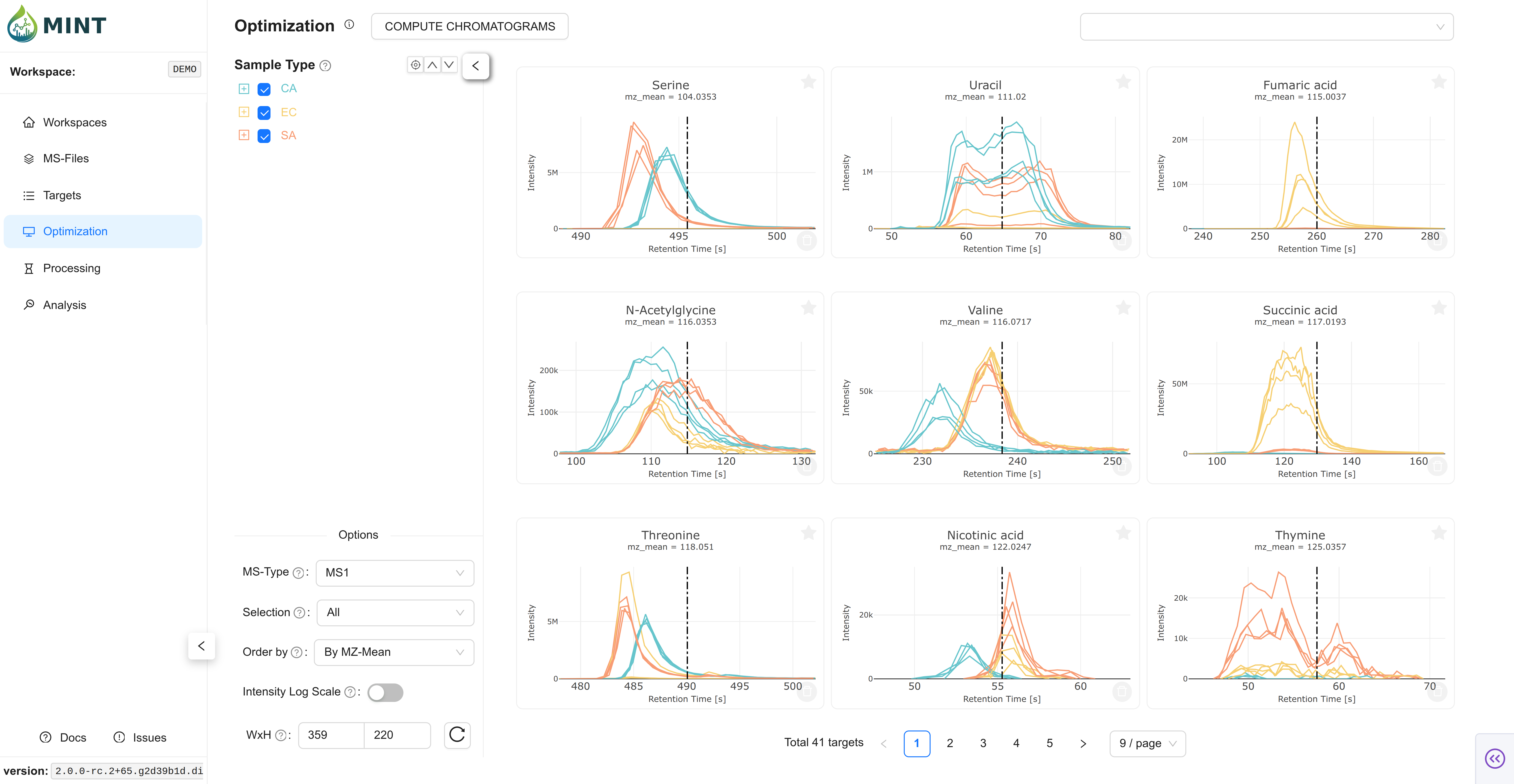
This shows the shapes of the data in the selected regions as an overview. It is a great way to validate that your target parameters are correct. However, you have to make sure the metabolite you are looking for is present in the files. That is why you should always include some standard samples (samples with the metabolite of interest at different concentrations). The colors in the plots correspond to the sample type colors in the metadata table.

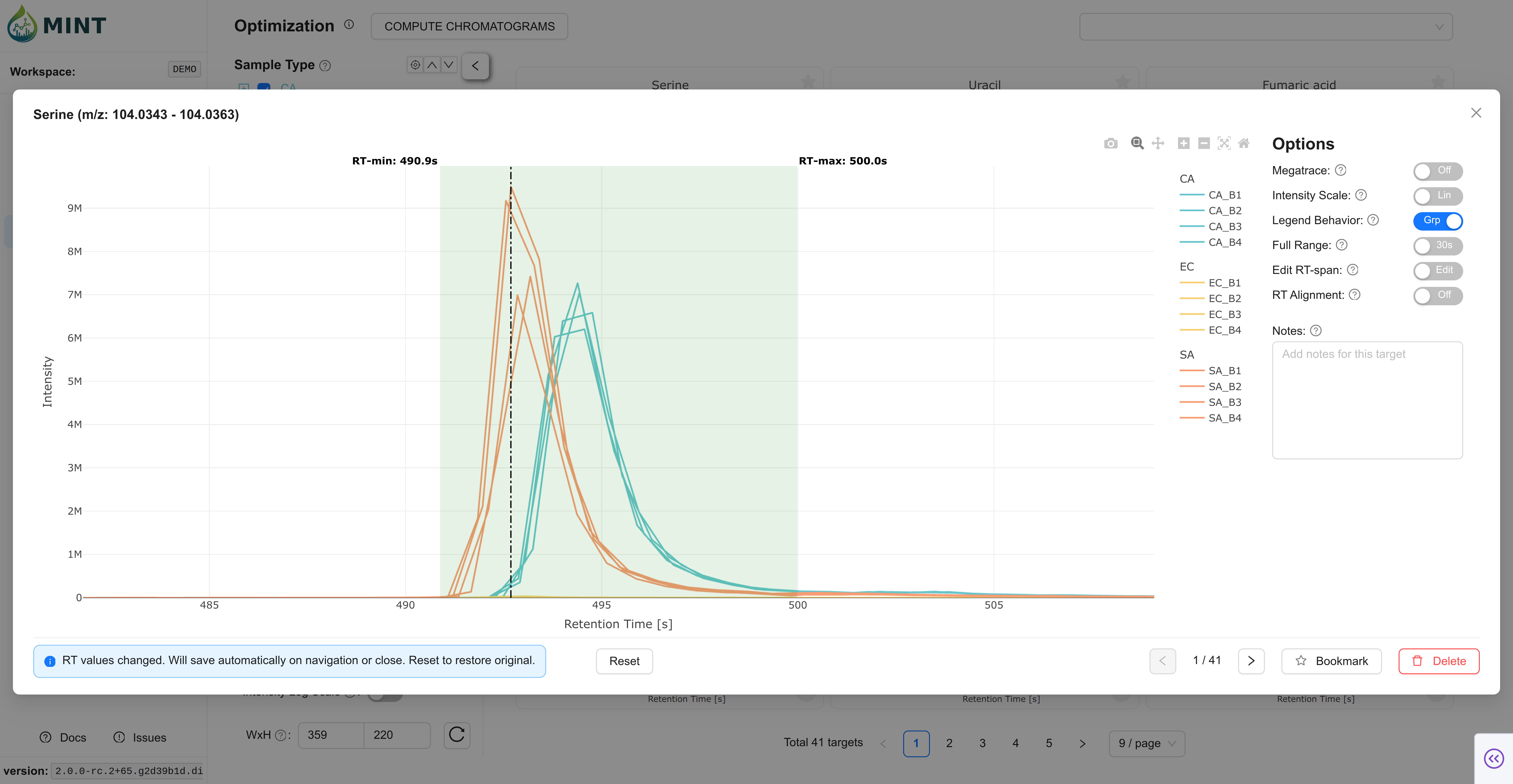
You can click on a card to use the interactive tool below and manually optimize the region of interest (ROI) or retention time span for each target. Move the borders of the box to select the peak, then click Save. The green area shows the currently selected retention time (RT) range. If the target is not present in any of the files, you can remove it from the target list by clicking Delete target.

Once the optimization is done, you can proceed to Processing.

8. Process the data

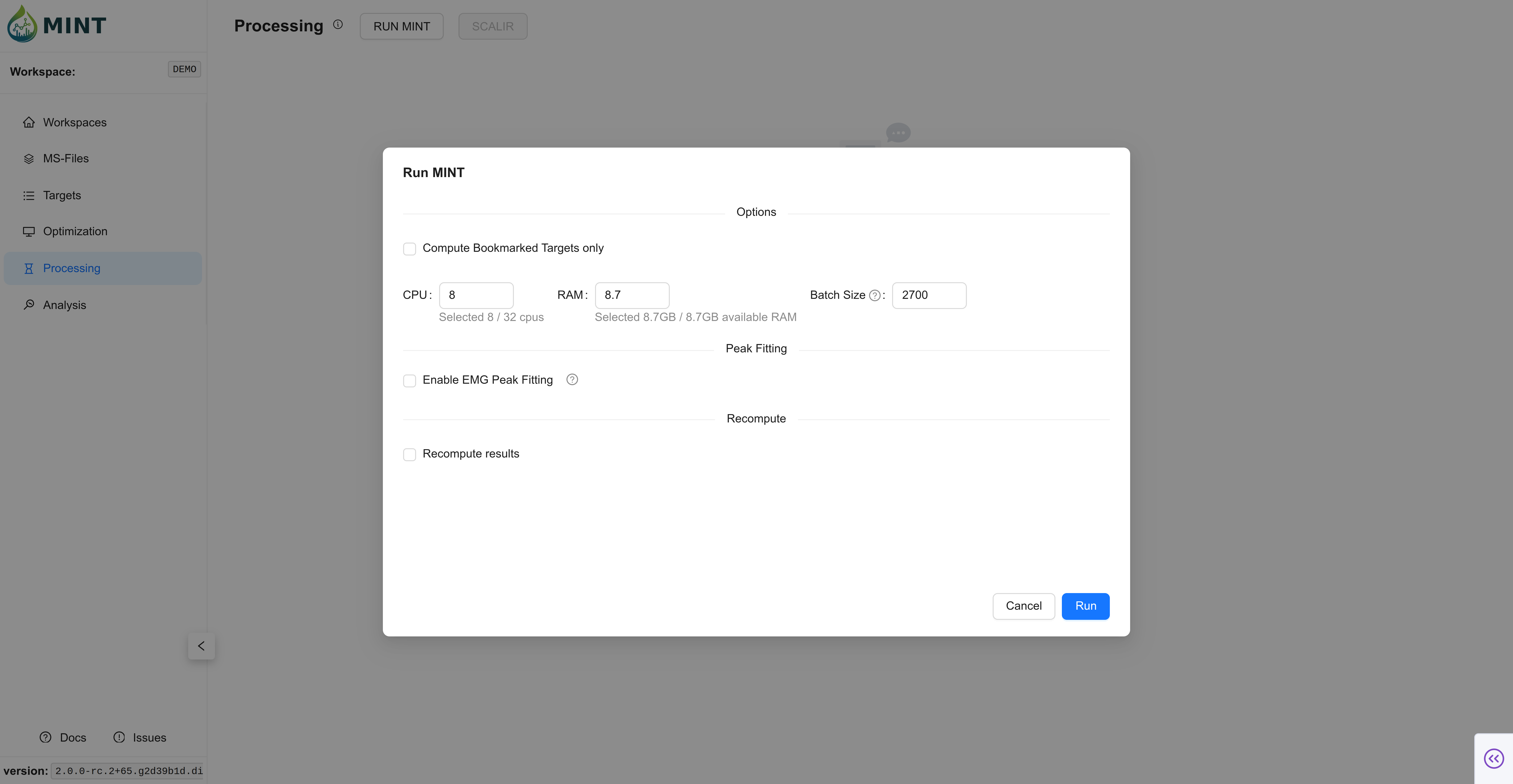
Switch to Processing and start data extraction with RUN MINT. As in Optimization, you can choose how many resources to allocate to process the files, including CPU, RAM, and batch size. In small datasets the default values should suffice; as the number of files grows, tweaking these parameters improves performance. Click Run to compute the results. For the demo data, this should take a few seconds-minutes depending on your machine.

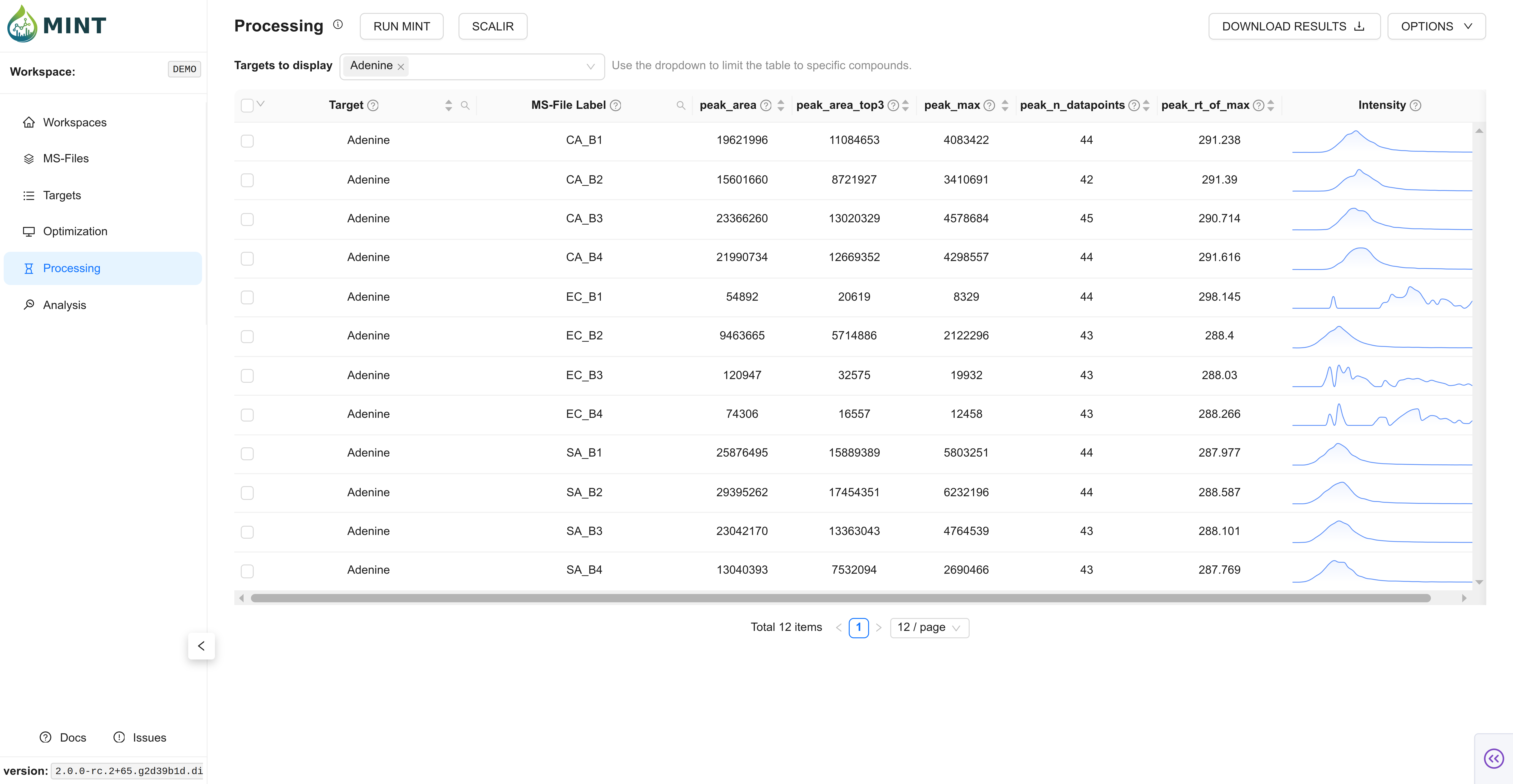
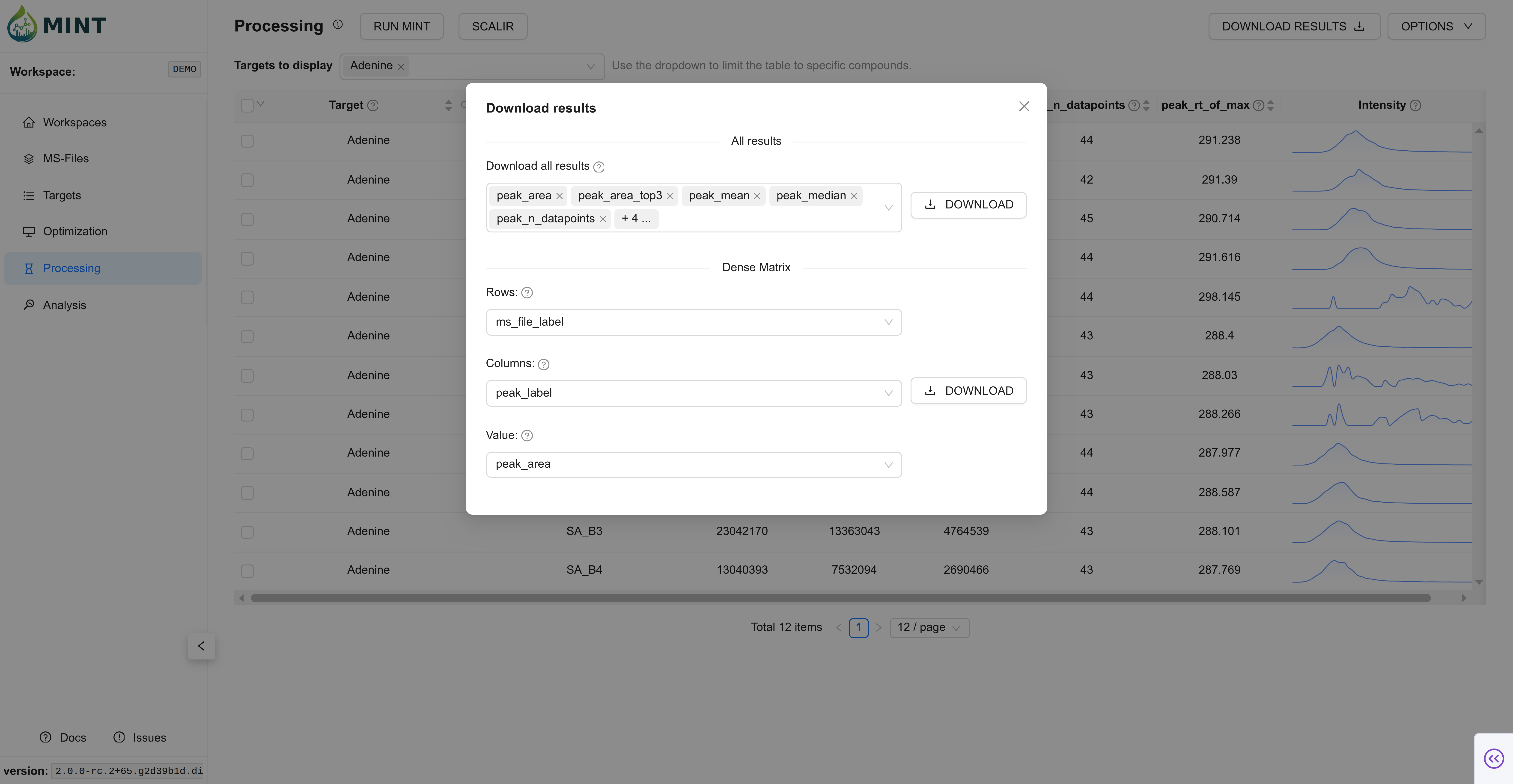
Now, you can download the results in long format or dense peak_max values by clicking DOWNLOAD RESULTS. The tidy format contains all results, while the dense format contains a selected metric (peak_max by default) as a matrix of values.

9. Analyze the results

Once the results are generated, there are several analyses you can perform. The Analysis section includes QC, PCA, t-SNE, Violin, Bar, Comparison, and Clustermap views. If you are new, start with QC to validate retention times and m/z stability, then use the Clustermap to quickly spot outliers or batch effects.

PCAt-SNEQCViolin (Distributions)BarComparisonClustermap (Heatmap)

Principal Component Analysis: Reduces the dimensionality of your data to visualize sample similarity.

Score Plot: An interactive scatter plot of samples projected onto Principal Components (PCs).
Cumulative Variance: Displays how much of the total dataset variance is explained by the first N components.
Loadings: A bar chart showing which metabolites contribute most to each PC.

t-Distributed Stochastic Neighbor Embedding: Nonlinear embedding to reveal local sample neighborhoods.

Axes: Select the t-SNE dimensions to display (typically t-SNE-1 vs t-SNE-2).
Perplexity: Adjust neighborhood size and regenerate to explore different structures.

Quality-control view for a selected target.

RT Plot: Retention-time stability across samples, grouped by your selected metadata column.
Metric Plot: Observed metric (e.g., peak area, peak area top3, etc.) across samples.
Chromatogram: Click a sample in either scatter plot to inspect the chromatogram for that target.
Progressive Loading: For large datasets, MINT initially loads a "Shadow Plot" (Envelope) to provide immediate feedback while detailed chromatogram data finishes loading in the background.

Focuses on the distribution of peak intensities for individual metabolites.

Selection: Use the dropdown to search for and select a specific peak.
Stats: Displays the distribution density and boxplots, grouped by your selected metadata column, along with ANOVA p-values for statistical significance.

Aggregated summary view by group.

Mean ± SEM: Bar chart with error bars.
Individual Samples: Jittered points overlaid on bars.
Chromatogram: Click a sample point to inspect its chromatogram.

Feature Comparison: Compare feature intensities between two selected groups using statistical tests.

Controls: Select two groups ("Sample 1" and "Sample 2") and set a P-value threshold and FDR correction method.
Plots: Toggle between a Scatter Plot (Mean vs Mean) and a Volcano Plot (Log2 Fold Change vs -Log10 P-value). Features meeting the significance threshold are colored.
Chromatogram: Click on any point in the plot to inspect the chromatograms for that feature across the two groups.

Displays a hierarchical clustering of samples (columns) and metabolites (rows). It helps identify patterns and outliers in your dataset.

Next steps

For a deeper tour of the interface, see the GUI guide.